Site perso : Emmanuel Branlard

• HOME
• Work
• Publications
• Contact
• Curriculum Vitae

• Papers
• Programs
• Music
• Linux
• Web sites

HOME workpapershtml2009fermi

3.2 Beam matrix and phase space

The understand the collective motion of a beam one require the trajectory of each single particle along with its momentum. To fully describe the state of a particle, and to describe it in a representative way, a six-dimmensional space is introduced: the phase space. Nevertheless, the knowledge of this coordinates for each single particle represent too much information, so that only the envelope of the beam is represented in the phase space. In practice, different curvatures can be found in the shape of the beam, nevertheless the canonical form chosen would be an ellipse and its representation by the so-called sigma-matrix.

3.2.1 Phase space

In the theory of beam physics, the three cartesian coordinates are not enough to fully describe the state of the particle, so that a system of 6 coordinates is used: $\left(x,x',y,y',s,\delta \right)$. Each coordinate being expressed with respect to the reference particle. Thus, unlike curvilinear coordinates, the coordinate $s$ is the longitudinal distance to the reference particle. This is the tricky part, when studying phase space coordinates, one has to keep in mind this definition. When confusion can be made, we will write these coordinates as: $(\tilde{x},\tilde{y},\tilde{s})$ to emphazise their relative definition. $x'$ and $y'$ represent the angle relative to their designed momentum. The transverse momenta $p_x$ and $p_y$ are also used. $\delta=\Delta p / p$ is the normalised momentum deviation. Energy deviation can also be used $\Delta E/E$ without significative difference remembering that $cp=\beta E$. This 6-dimensional space is called phase space and will be further used to study the evolution of the envelope ofa bunch through an accelerator. In absence of couplying between the different plane, the phase space may be split into three independant 2-dimensional phase planes. This hypothesis is often used, eventhough coupling terms are always present, and might sometime be significant.

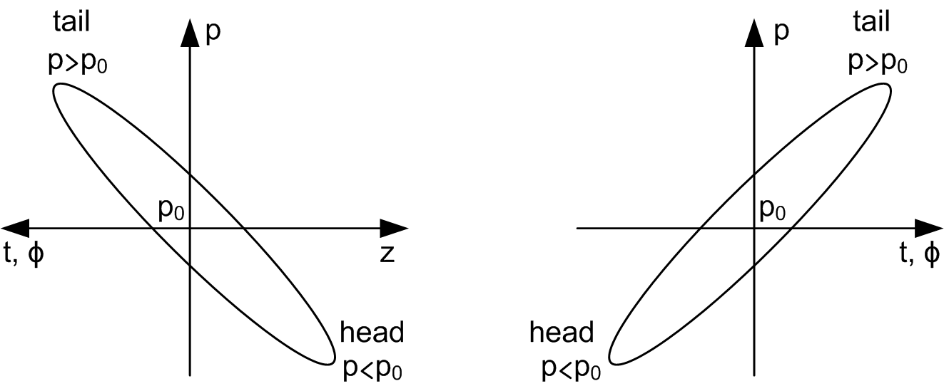
Two conventions exists for the longitudinal phase space. Indeed, let's consider a particle which is in front of the reference particle in term of the longitudinal coordinate: $z>z_0$. Then this particle will arrive before the reference particle, so its time of arrival is less than the time of arrival of the reference particle: $t<t_0$, or in term of phase $\Phi<\Phi_0$. This results in two different phase space representations as one can see on figure 3.2. To go from one representation to the other we just have to flip the scheme horizontally. As a result of this, the shape of the ellipse is modified. If one is not careful, this could lead to completly different interpretations while analyzing a phase space sheme. In Astra, an in the rest of this document the ''z convention`` will be used.

Figure 3.2: Different convention for the longitudinal phase space. (left) Convention used by astra and further in this document: $z$ is is used as reference - (rigth) Convention using the difference of phase, or arrival time with respect to the reference particle

3.2.2 Beam emittance

Each particle of a beam is a point in the phase space. The envelope of all these points represents the region occupied by the beam in phase space. This region is called beam emittance, and its value is normalized proportionally to the surface area. In the case of absence of coupling between the different phase plane, three independent beam emittances are defined. In each plane, the region delimited by the particles will be represented by an ellipse for its easy analytical description. The general equation of a 2D phase space ellipse is:

$$\gamma x^2 + 2\alpha x x' + \beta x'^2 = \epsilon$$ (3.7)

The notation $\alpha, \beta, \gamma, \epsilon$ are commonly used. They indeed recall the notations used when we introduce the betatron functions, the Courant-Snyder invariant, and the Twiss-paramters in section 2.2. From geometric properties of an ellipse we have the relation:

$$\beta \gamma -\alpha^2 =1$$ (3.8)

The area defined by this two dimensional ellipse is:

$$A = \int_{\text{ellipse}} dx dx' = \pi \epsilon$$ (3.9)

The emittance, for instance in the plane $(x,x')$, can be expressed as the root mean square value (rms):

$$\epsilon_x=\sqrt{\langle x^2\rangle \langle x'^2\rangle-\langle xx'\rangle^2} = \sqrt{\sigma_x^2 \sigma_{x'}^2-\sigma_{xx'}^2}$$ (3.10)

Nevertheless, the canonical parameters related to each other are $x$ and $p_x$, instead of $x$ and $x'$. As a result of this, a normalised emittance is defined as:

$$\epsilon_{nx}=\frac{1}{m_0 c}\sqrt{\langle x^2\rangle \langle p_x^2\rangle-\langle xp_x\rangle^2}$$ (3.11)

The relation between the two is:

$$\epsilon_{nx}= \beta \gamma \epsilon_x$$ (3.12)

3.2.3 Beam matrix

The general equation of an $n$-dimension ellipse can be written as:

$$u^{T} \Sigma^{-1} u = 1$$ (3.13)

where $u \in \Re ^n$ and $\sigma \in \Re ^n \times \Re ^n$. The ellipse volume is:

$$V=\frac{\pi^{n/2}}{\Gamma(1+n/2)}\sqrt{\det\Sigma}$$ (3.14)

In the context of phase space, a maximum of six dimensions will be used with $u = \left(x,x',y,y',z,z'\right)^T$. The $\Sigma$-matrix will be also called the beam matrix

3.2.4 Two dimensional beam matrix - Relation with Twiss-parameters

The equation of the phase space ellipse in $\sigma$-notation is as following

$$u^T \Sigma^{-1} u = \frac{1}{\det(\Sigma)} \left[ \sigma_{22} x^2 -2 \sigma_{12} x x' + \sigma_{11} x'^2\right] =1$$ (3.15)

Let's identify it with the previously introduced equation of the ellipse in Twiss-parameters:

$$\gamma x^2 + 2\alpha x x' + \beta x'^2 = \epsilon$$ (3.16)

The link between these two equation can be obtained by equaling the two ellipse areas:

$$\frac{A}{\pi} = \sqrt{\det\Sigma} =\sqrt{\sigma_{11}\sigma_{22}-\sigma_{12}^2} \ \ \ \ \ \ \ \ \ \ \frac{A}{\pi} =\epsilon$$ (3.17)

This leads to the following relation:

$$\Sigma = \begin{pmatrix}{\it\sigma_{11}} & {\it\sigma_{12}}\\ {\i... ...rix} = \epsilon \begin{pmatrix}\beta &-\alpha\\ -\alpha& \gamma\\ \end{pmatrix}$$ (3.18)

One has to be carefull not to be confused between elements of the $\Sigma$ matrix, and the standard deviation their are related to: $\sigma_{11}=\sigma_{x}^2$ , $\sigma_{22}=\sigma_{x'}^2$ and $\sigma_{12}=\sigma_{xx'}$. For this reason, we will explicitly write down the relations described by equation 9.7 and schematize their geometrical intepretation in figure 3.3.

$$\sigma_x = \sqrt{\epsilon \beta}\ \ \$$ (3.19)

$$\sigma_{x'} = \sqrt{\epsilon \gamma}\ \ \$$ (3.20)

Figure 3.3: Graphical representation of the Twiss-parameters

3.2.5 Relation with transport matrix

If the transportation matrix from a point 0 to a point 1 is known, then the beam matrix a point 1 $\Sigma_1$ can be related to the beam matrix at point 0 with the following relation:

$$\Sigma_1 = M \Sigma_0 M^T$$ (3.21)

Given an input sigma matrix, one can try to find which succesion of elements will provide a transportation matrix $M$, such that the output sigma matrix will satify specific requirements.

3.2.6 Four dimensional beam matrix - introduction to Emittance exchange

To simplify the study of the beam matrix evolution as it propagates through a beam line, we will assume the initial beam matrix to be diagonal by block:

$$\Sigma_{in}= \begin{pmatrix}\Sigma_x&0\\ 0&\Sigma_z\\ \end{pmatrix}$$ (3.22)

Emittance exchange is complete if after a tranformation, the output sigma matrix is of the form :

$$\Sigma_{in} \approx \begin{pmatrix}\Sigma_z&0\\ 0&\Sigma_x\\ \end{pmatrix}$$ (3.23)

Writting the transportation matrix $M$ in a general form:

$$M=\begin{pmatrix}{\it a_{11}} & {\it a_{12}} & {\it b_{11}} & {\i... ...{21}} & {\it d_{22}} \\ \end{pmatrix} =\begin{pmatrix}A&B\\ C&D\\ \end{pmatrix}$$ (3.24)

Equation 3.22 results in:

$$\Sigma_{out}=\begin{pmatrix}A\Sigma_xA^T + B\Sigma_zB^T & A\Sigma... ...D^T \\ C\Sigma_xA^T + D\Sigma_zB^T &C\Sigma_xC^T + D\Sigma_zD^T\\ \end{pmatrix}$$ (3.25)

Complete emittance exchange is reached if $A=0\ \&\ D=0$

Emmanuel Branlard
http://emmanuel.branlard.free.fr/