Site perso : Emmanuel Branlard
Next: 14.2 An example of transportation matrix: five cell | Up: 14. Study of a cavity | Previous: 14. Study of a cavity |
Navigation: Contents | Index
- 14.1.1 Longitudinal component
- 14.1.2 Correlation introduced by a cavity between
 and the energy
- 14.1.3 Determination of the cavity matrix
14.1 Fields inside a cavity
14.1.1 Longitudinal component
In its most general form, the solution of the wave equation is expressed with Bessel functions. For a| (14.1) |
where
14.1.2 Correlation introduced by a cavity between and the energy
Lets introduce a bunch into the cavity and determine its gain in energy. The field seen by a particle P when it is at a position 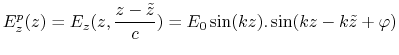 |
(14.2) |
The hypothesis of relativistic speed imply that ![]() is a constant for a given particle. We will thus introduced the phase
is a constant for a given particle. We will thus introduced the phase
![]() with
with
![]() . This traduce that the difference of arrival time in the cavity between the particles of the bunch can be expressed by a difference of phase in the expression of the field.
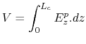
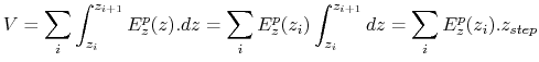
The total energy gained by a particle during its travel through the caviy is then obtained by calculating the following integreal:
. This traduce that the difference of arrival time in the cavity between the particles of the bunch can be expressed by a difference of phase in the expression of the field.
The total energy gained by a particle during its travel through the caviy is then obtained by calculating the following integreal:
![$\displaystyle \int_{z=0}^{z=l_c} \left[ \cos(\phi)-\cos({2kz+\phi}) \right]dz = \frac{1}{2k}\left[ \sin(\phi+2kl_c)-sin(\phi) \right] +l_c \cos(\phi)$](img644.gif) |
(14.3) |
But as the design of a cavity is such that the length of the cavity
| (14.4) |
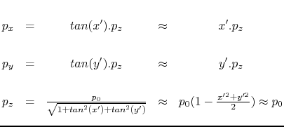
Thus, for the reference particle:
| (14.5) |
The difference of the two last expression, gives us the evolution of the energy space phase coordinates through the cavity:
| (14.6) |
Or, by writting this expression in term of momentum:
| (14.7) |
Expression in which we can see that a linear dependence has been introduced by the cavity between the momentum and the longitudinal coordinate. The slope of this correlation,
 (a)
(a)
 (b)
(b)
14.1.2.1 The fields time phase
The fields we have is a picture of the time depending fields. To make them be time dependent astra will multiply them by a time depending sine function. The same is done for the other components of E and B. As we included in our field map the two small pipes surrounding the cavity, the best way to adjust the phase is to adjust it in reference to the middle of the cavity. Indeed, at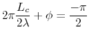 |
(14.8) |
We find

14.1.2.2 The fields scaling
As the fields were generated by , arbitrary values of the power given to the cavity were inputed. As a result of this, the fields have to be scaled to their real values by multiplying all the E and B components by a same scaling factor. Astra has his own scale factor algorythm, but it uses the maximum E value on the cavity axis. With the
 |
(14.9) |
Numerically we have data every
 |
(14.10) |
We find
![]() V/m, and a scale of 9.3227e+6 to have the good field amplitude in V/m, which means a scale of 9.327 to have a field in MV/m which is what is expected by ASTRA. We will use the same scale factor for B, which will give us fields in MTesla, which is an non usual unit, but it seems that it is what is needed by astra. As our hfss field map represent H, we will also multiply this by
V/m, and a scale of 9.3227e+6 to have the good field amplitude in V/m, which means a scale of 9.327 to have a field in MV/m which is what is expected by ASTRA. We will use the same scale factor for B, which will give us fields in MTesla, which is an non usual unit, but it seems that it is what is needed by astra. As our hfss field map represent H, we will also multiply this by ![]() .
.
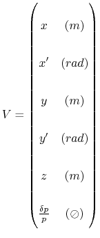
14.1.3 Determination of the cavity matrix
14.1.3.1 Notation used for the cavity
In the previous section, we used
This will be useful when we will further need to go from
Next: 14.2 An example of transportation matrix: five cell | Up: 14. Study of a cavity | Previous: 14. Study of a cavity |
Navigation: Contents Index